Fitting psychmetric functions
General principle
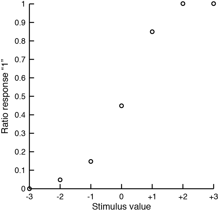
Fitting psychometric functions is one of the most useful skills in psychophysics. The basic statement of the problem is as follow: given a set of observations $R$, one wants to recover the parameters $\Theta$ that are most likely to have generated the observation. Or: $$\underset{\Theta}{Argmax}\ \mathcal{L} (R|\Theta)$$ This equation simply means we want to find the values of $\Theta$ that maximizes (argmax) the likelihood function $\mathcal{L}$ of $R$ given $\Theta$. What is the likelihood function? The likelihood function is the probability to have observed the data given the parameters. The data contains many trials $R = (r_1,r_2,\dots,r_N)$, which have values 0 or 1. Here 0 or 1 does not mean correct or incorrect, but the response to the task (e.g. is it tilted to the right or left, is it green or red...). So the likelihood function is the probability to have observed all these values given the parameters. Or: $$\mathcal{L} (R|\Theta) = p(R|\Theta) = p(r_1,r_2,\dots,r_N|\Theta)$$ Usually we assume that the psychometric function is a cumulative normal function, or $\Phi$. We also assume that trials are independent. The probability to observe two independent events is simply the product of the probability of each event: $p(x,y)=p(x)p(y)$. $$p(R|\Theta) = p(r_1,\dots,r_N|\Theta) = p(r_1|\Theta)p(r_2|\Theta)\dots p(r_N|\Theta)$$ To restate the problem: $$\underset{\Theta}{Argmax}\ \prod_{i=1}^{N} \Phi(r_i|\Theta)$$ This equation simply means we want to find the values of $\Theta$ that provides the highest possible product of probabilities to have observed individual trials $r_i$, when these values are generated by a cumulative normal function. Let's say you collected trials on a task. The dependent variable had 7 values $(-3,-2,\dots,+3)$. And you collected 20 trials for each of these values. Your observations are: $R=(0,1,1,0,0,1,\dots)$, corresponding to stimulus values $V=(-2,+1,0,-1,-3,+2,\dots)$. When you plot the ratio of trials where an observer answered "1", you get something like this:
Optimization
All that remains to be done is to find $\mu$ and $\sigma$ through optimization.
Luckily, you don't have to worry too much about this part and can use one of the great algorithms that already exist.
The most popular is the Nelder-Mead "simplex" algorithm.
A good alternative is one of the many quasi-Newtonian gradient descent.
In matlab these are implemented in respectively the fminsearch and fmincon functions.
There is one last mathematical step to make before to use optimization.
Because all probabilities are between 0 and 1, by definition, their product will very quickly become extremely small.
And computers are not very good at handling small numbers.
This can be avoided using the logarithm function.
This function will transform the probabilities into a negative number.
Moreover, one of the properties of logarithms is that $log(x.y)=log(x)+log(y)$.
Logarithms transform multiplications into additions, which is what makes them so great.
So instead of optimizing the product of all probabilities, it is more convenient to optimize the sum of their logarithms.
Or:
$$log \left(\prod_{i=1}^{N} \Phi(r_i|\Theta)\right) = \sum_{i=1}^{N} log \left(\Phi(r_i|\Theta)\right)$$
Finally, optimization algorithms try to find the minimum of a function.
Here we want to find the values of $\Theta$ that maximizes the likelihood $\mathcal{L}$.
This can be done by minimizing $-\mathcal{L}$.
So we will use an optimization algorithm to find the values of $\mu$ and $\sigma$ as follow:
$$\underset{\Theta}{Argmin}\ - \sum_{i=1}^{N} log \left(\Phi(r_i|\Theta)\right)$$
The function we try to minimize is called the objective function.
Here are two programing tricks for matlab.
First, remember that we want to use $p(r_i)$ when the answer was 1 and $1-p(r_i)$ when the answer was 0.
Because responses $r_i$ are 0 or 1, multiplying the probability of the response with the response will be 0 when the answer is 0, and $p(r_i)$ when the answer is 1.
Similarly multiplying $1-p(r_i)$ by $1-r_i$ will be 0 when the answer was 1 and $1-p(r_i)$ when the answer was 0.
So if we put the stimulus values $V=(v_1,\dots,v_N)$ and responses $R=(r_1,\dots,r_N)$ into vectors:
$$V=\begin{bmatrix} v_1 \\ \vdots \\ v_N \end{bmatrix} \qquad R=\begin{bmatrix} r_1 \\ \vdots \\ r_N \end{bmatrix}$$
Then we can compactly compute the probabilities of each response in matlab as:
R.*normcdf(V,mu,sigma) + (1-R).*(1-normcdf(V,mu,sigma)
In matlab .* is the pointwise operation ($\circ$ in vectorial notation), or the multiplication of each value of the vector by the correspnding value of the other vector ($r_i.p(r_i)+(1-r_i).(1-p(r_i))$).
Secondly, we can use anonymous functions to compactly compute the objective function.
Anonymous functions work like functions but can be declared inside a script or another function in a single line of code.
Anonymous functionsare declared by their name, followed by = @(...) with the function parameters inside the parentheses, followed by the function itself.
For example:
anonymousfunction = @(x,y) x+y;
This anonymous function is called by result = anonymousfunction(variableA,variableB) and will return the sum of variableA and variableB in the variable result.
We can write our objective function inside an anonymous function:
fitfun = @(theta,data) -sum(log(data(:,2).*normcdf(data(:,1),theta(1),theta(2))+(1-data(:,2)).*(1-normcdf(data(:,1),theta(1),theta(2)))));
To call this function, we put the stimulus values and responses into a 2-columns matrix, with the stimulus values in the first column and the responses in the second:
$$data = \begin{bmatrix} v_1 & r_1 \\ \vdots & \vdots \\ v_N & r_N\end{bmatrix}$$
Or in matlab D=[V,R], where V and R are column vectors with respectively the stimulus values and responses.
We also put the 2 parameters $\mu$ and $\sigma$ in a vector $\Theta=\begin{bmatrix}\mu & \sigma\end{bmatrix}$.
This function will compute the probability $p(r_i)$ that each response is "1" (or "0") according to the stimulus values, $\mu$ and $\sigma$, multiply it by the response $r_i$ (or $1-r_i$), as described above.
Then it will take the logarithms of all these probabilities and return the inverse of their sum.
All in 1 line of code.
Now we are ready to use an optimization function.
We will use fminsearch.
This function requires starting values $\Theta_0$.
Lets start with $\mu_0=0$ and $\sigma_0=1$.
In matlab this is theta0=[0,1].
The data must be passed to the function as optional arguments.
We call it like that:
thetahat = fminsearch(fitfun,theta0,[],D)
Here $\hat{\Theta}$ are the estimated parameters.
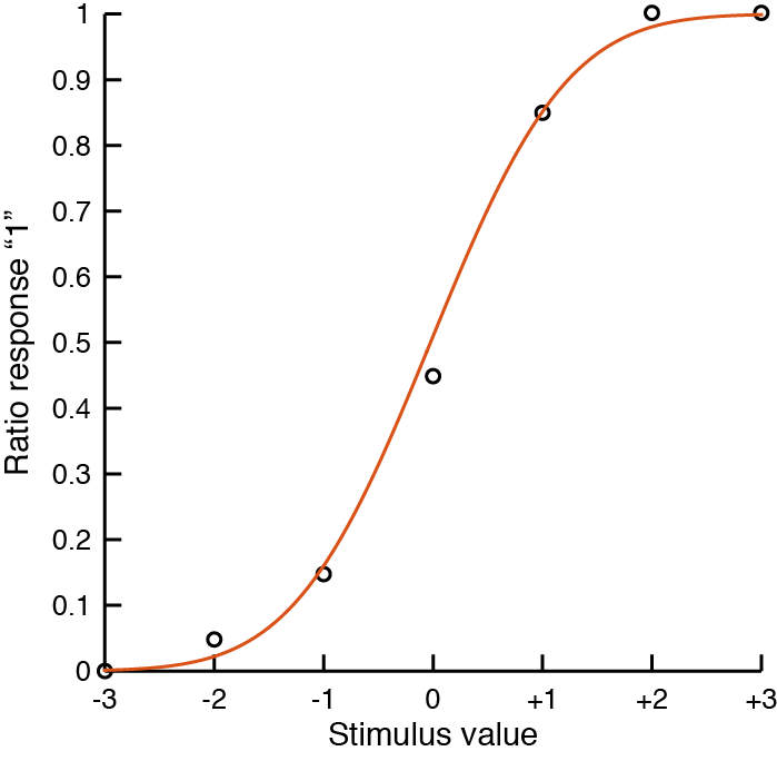
For the data plotted above, fminsearch returns thetahat = -0.0238 0.9823.
Plotting a cumulative normal function with these parameters show that this is a very good fit:
fitfun = @(theta,data) -data(:,2)'*log(normcdf(data(:,1),theta(1),theta(2)))-(1-data(:,2))'*log((1-normcdf(data(:,1),theta(1),theta(2))));Which does exactly the same thing.
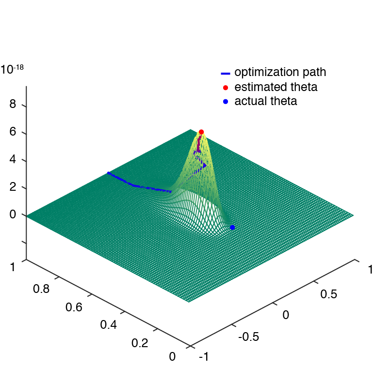
Likelihood surface
Plotting the likelihood surface helps to understand how the optimization algorithm works.
Here is the script that generates a likelihood surface.
Run the script psychfunfit_demo.m.
More parameters
In practice, it is often desirable to use more than 2 parameters.
In particular, observers sometimes have lapses: trials where they press the wrong button by accident.
With only 2 parameters, observers are assumed to reach 0% or 100% when stimulus values become extreme.
In practice this can lead to an underestimationof the slope of the psychometric function.
Assuming that observers have as many lapses for low and high stimulus values, the psychometric function becomes:
$$f(v_i)=\frac{\lambda}{2}+(1-\lambda)\Phi(v_i|\mu,\sigma)$$
Where $\lambda$ is the lapse rate.
One problem introduced by the lapse rate is that the optimization algorithm can estimate the objective function using negative values.
This will lead to probabilities higher than 1 or lower than 0.
There are 2 ways to avoid this problem.
We can use the function fmincon, which uses a different optimization than fminsearch, and allows for constraints.
We can keep $\mu$ and $\sigma$ unconstrained (that is put $-\infty$ and $+\infty$ as limits), and keep $\lambda$ between 0 and 0.5.
Alternatively we can transform $\lambda$, using for example the exponential function, to ensure that it will be positive.
This way, even when the optimization function calls the objective function with a negative value for $\lambda$, it will then be converted to a positive value.
You can also do that for $\sigma$.
Finally, to also put a maximum value you can use a different function such as the cumulative normal.
Confidence intervals and resampling
Ultimately, you'll probably do statistics across-observers on the fitted parameters. But it is also useful to do within-observer statistics. This can be done with resampling, more specifically boostraping. In boostraping, the dataset is treated as the population. Then new samples are simulated by randomly selecting trials from the dataset with replacement. As if the experiment was performed again but on the sampled data. Then a psychometric function is fitted on each resample. Confidence intervals can be estimated from the distribution of fitted parameters by finding parameter values that contains 95% of the parameters. Bootstraping requires a large number of resamples, idealy millions. When fitting psychometric functions, which takes time, a reasonable number of resamples is 10000. For example, bootstraping the data above gives a confidence interval for $\mu$ of [-0.44,0.31].
Fitting other functions
Ratio correct
N-AFC
Response times
Confidence
Fitting multiple functions
Fitting with priors